Expertise:
Beginner
Functional Analysis of Variance - Continued
An important part of building a linear model is to assess the fit by examining the residuals and calculating
the percent variance explained by the model. The functional linear model is no different; the residuals
are a function of time and can be plotted, and functional analogues of the R2 and
F-ratio can be calculated.
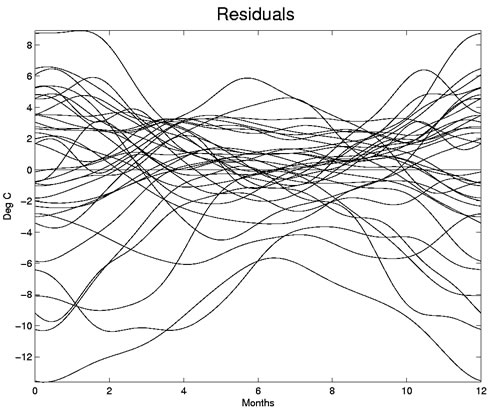
Figure 3: The residual functions for the functionalanalysis of variance.
Residual points have a random scatter in a classical linear model with a good fit to the data; we
would expect our residual functions to also display a randomness and be centered about zero. This is the
case here, although there are a few negative outliers, especially in the summer months.
The R2 and F-ratio functions are plotted below. The R2 value is
above 0.5 throughout the year, indicating a good fit. The linear model is particularly good at explaining
the variability in the spring and autumn months, since this is where the climate zones most differ. The few
outlying residuals in the summer months would also contribute to a lower R2. The
F-ratio function parallels the R2 function and is substantially
above the 5% significance level at every point in the year.
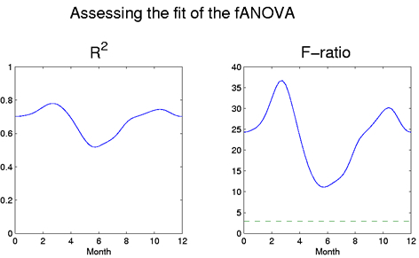
Figure 4: The R2 and F-ratio functions for the
functional analysis of variance. The horizontal
dotted line on the right panel indicates the
5% significance level for the
F-distribution with the appropriate degrees of freedom.
What have we learned?
These weather data provide an excellent basis for exploring some basic ideas of functional data analysis,
including:
functional summaries of the data, such as mean, standard deviation, and correlation, functional principal components, and functional linear models, such as the ANOVA.
We saw in the weather example that there exist functional analogues of classical multivariate statistical summaries
and methods. One of the strengths of FDA lies in its ability to easily adapt traditional methodology
into a functional framework, giving researchers a familiar environment for analysis and interpretation.
The results of these functional analyses are best interpreted through plots. Through graphical displays
we can easily see how classical analyses are extrapolated into the functional realm - we can notice how
the computed regression coefficients vary over time, for instance, and we can also spot subtle transient
effects to explore with further analyses.
|